Boris is the CEO of Census. Previously, he was the CEO of Meldium, acquired by LogMeIn. He is an advisor and alumnus of Y Combinator. He enjoys nerding out about data and technology, 8-bit graphics, and helping other startup founders.
What does lead scoring really mean?
The problem is common: your team has many potential customers but not enough bandwidth to pursue them all. Whether you are a product led business with tons of freemium users, have a great inbound funnels of leads or simply an amazing SDR team booking meetings, at the end of the day, you need to prioritize the time of your sales teams and give them the “best” leads. This is true for any type of leads, Marketing Qualified Leads, Sales Qualified Leads or my favorite: Product Qualified Leads.
So how do you evaluate leads and route them to your sales to maximize win rate?If your customer base is small, you may have some intuition as to which leads are likely to convert into a sale. But for a business looking to scale, it's inefficient (and eventually impossible) for a human to eyeball each lead and make a gut decision.
Cue lead scoring, in which a set of rules assigns each new lead a priority in your queue. These rules are developed by looking at which kinds of leads have converted to sales at the highest rates in the past. In other words, lead scoring depends on having a predictive model for lead conversion.
Depending on your organization’s needs, lead scoring may not always be the right answer. If your pool of customers is relatively small but each sale is high-value, it may be worth it for a human to go through each potential lead and make a manual prioritization. This would allow you to incorporate information that may be hard to systematically quantify, like the strength of your social and professional networks with each potential customer and the positioning of competitors who may be vying for the same contracts.
As a rule of thumb, the smaller the value of each sale compared to your total bottom line, the more important it is to process leads quickly, and the less it makes sense to dedicate an employee to understanding and assessing hard-to-quantify factors.
In these cases, scoring leads via conversion models can substantially improve your sales revenue while reducing costs.
What's a model?
A model relates a single outcome variable to any number of explanatory variables by looking at patterns in historical data. Lead scoring is based on predictive modeling, where rules can be used to decide if a lead is ready to be engaged by your sales team.
Predictive modeling is the focus of this post, but it’s also worth mentioning causal modeling, which focuses on determining which factors are effective in influencing outcomes. This could be useful for determining which kinds of sales strategies are most effective, but it’s not useful for predicting conversion of new leads. We’ll cover causal modeling in a future post.
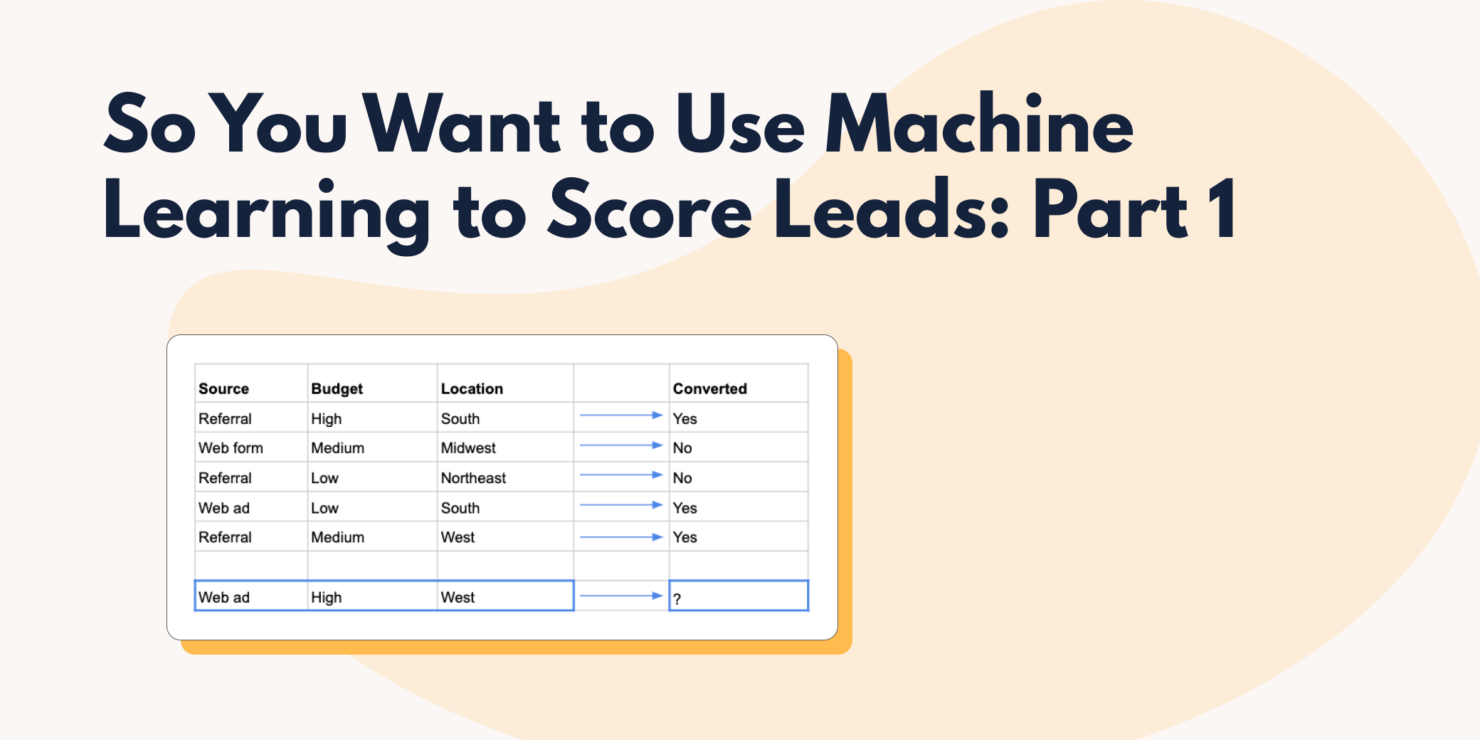
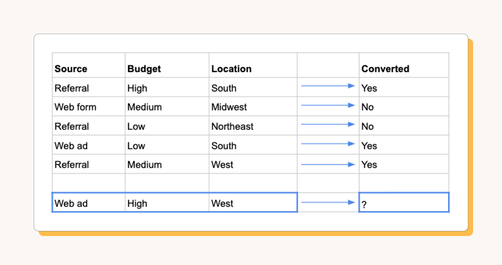
In lead scoring, our data might look something like this:
Outcome variable:
Converted: whether or not a lead converted to a sale
Explanatory variables:
Source: how we got the lead
Budget: the potential customer's estimated budget
Location: the region where the potential customer is based
What if my data is more complex than convert vs. not convert?
A binary (true/false) conversion status may not fit perfectly with the way your leads are structured. However, many seemingly complex structures can be boiled down to true/false outcomes. Say you offered a tiered plan for your product, and you wanted to predict which users are likely to move from your free tier to your basic tier, or from your basic tier to your premium tier in some billing cycle.
You could break this into two models: one modeling whether free users move to basic (“true”) or stay in free (“false”), and a completely separate model for basic vs. premium. Of course, binary models can’t answer questions like “how long is a given user likely to stay before churning?” or “how much revenue is a given lead likely to generate?”. We’ll cover when and how to model more complex outcomes in future posts.
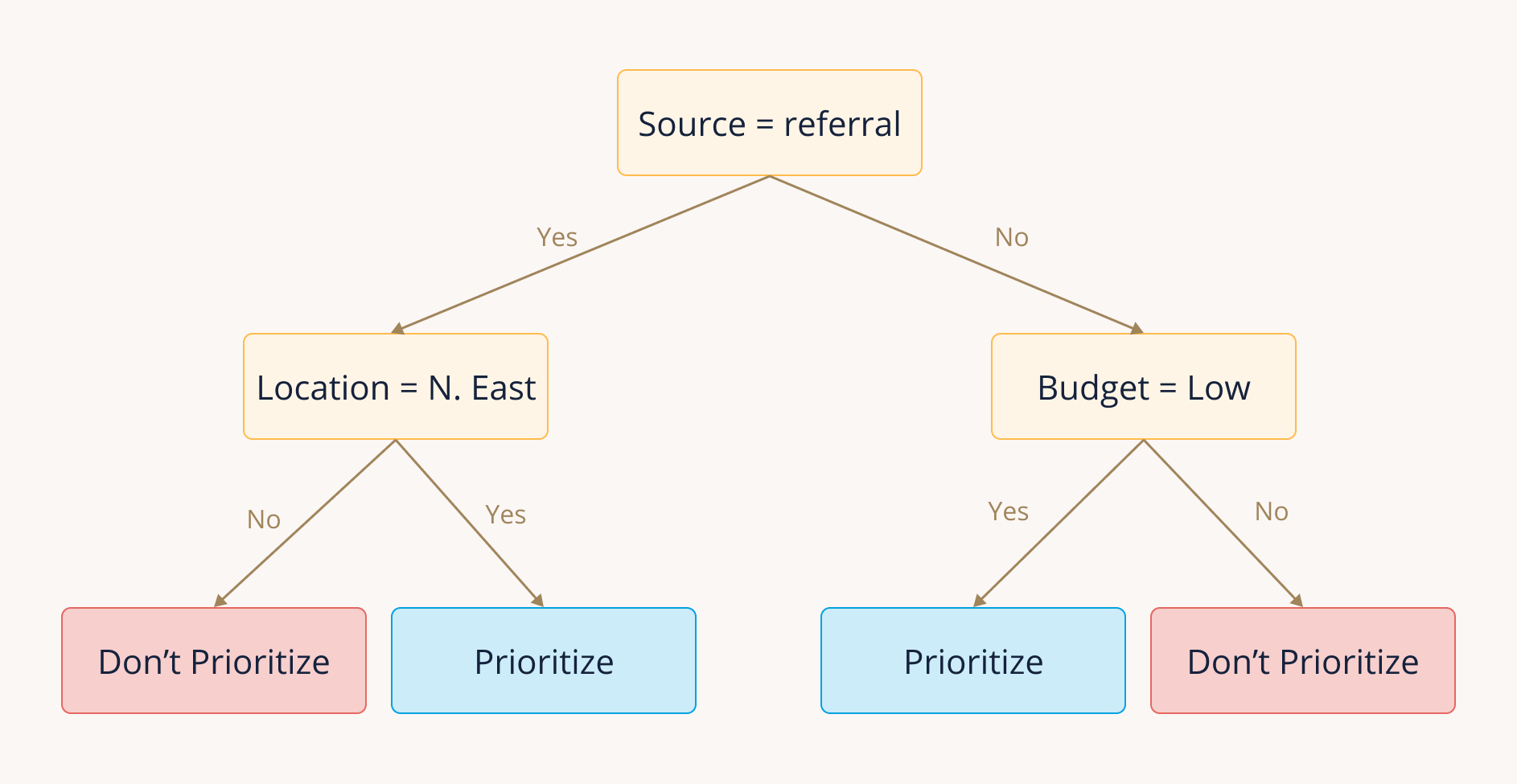
Most models used in practice are based on rules-of-thumb that humans have learned through experience. For example, we might notice over time that leads with Source = "referral" seem more likely to convert than leads from other sources. We can use this information to prioritize following up on new leads that come from referrals. Our assumption is that patterns we've observed in the past will continue to hold for new leads.
Many organizations end up building a collection of these heuristics over time, and they use them as a strategy to triage new leads. A set of heuristics can often be represented as a decision tree, or a series of true/false statements that someone can follow to make a consistent prediction about the outcome of a new lead. Using our example variables from above, we might end up with a decision tree like this:
How does all this relate to machine learning?
The simple, heuristic-based model described above may be insufficient when:
Lead volume is high
Response time has to be fast
There are many potential explanatory variables
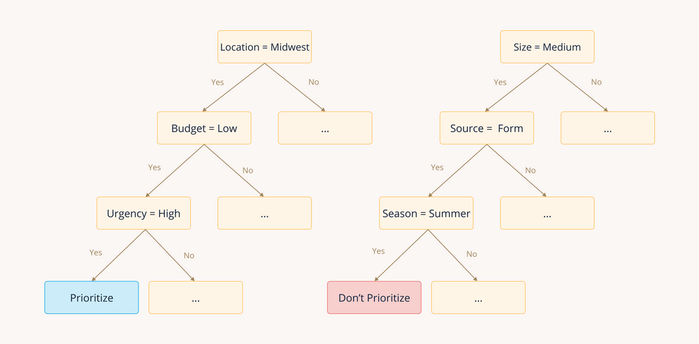
In these cases, manually scoring each lead becomes unsustainable, and heuristic-based models start to fall apart.Let's say that in addition to our explanatory variables listed above, we also have the variables Season, Urgency, and Size. We start to notice that:
Leads from the Midwest with low budget but high urgency have converted 80% of the time.
Leads from medium-sized companies that were submitted via a web form during the summer have only converted 20% of the time.
These may be real patterns in the data, but which outcome would we guess when we receive a new lead from a medium-sized, Midwestern company with low budget and high urgency that submitted a web form during the summer?
It would be infeasible for a human to comb through every possible combination of these 6 explanatory variables to make rules for each, let alone if there were hundreds of features with countless new leads generated every day.
This is becoming the norm for SaaS companies, where every user action in-app is tracked, and any of these features might predict conversion, spend, or churn.
This is where supervised machine learning models come in, and they're often straightforward to implement using free, open-source code. Here's the catch: no matter how well-designed an ML algorithm is, it's useless without good data.
How can I tell if my data is "good"?
It's an open secret that the hardest part of data science in the real world isn't building a good ML model; it's dealing with the raw data before it ever touches the model.
What makes data good or bad depends on what we want to do with it, and data management is so complex that it’s standard to have an entire team dedicated to it. For now, let's highlight the key features that make data good for lead scoring specifically.
1. Data should be stored in a standardized way.
Broadly, all data on past leads and conversions should be kept in a consistent, accessible place. For ad-hoc models with limited sample size, storing data directly in Excel might be okay. But for production models, where a process needs to be automatically rerun on new data, we'll need a scalable, schema-enforced solution.
In other words, each data point on a lead should always follow the same format with the same data types; for example, every lead might be forced to have a CreateDate value that's always in the format YYYY-MM-DD.
2. Data should be snapshotted.
One of the most common mistakes in predictive modeling is allowing target leakage, where information "from the future" is accidentally introduced into our explanatory variables.
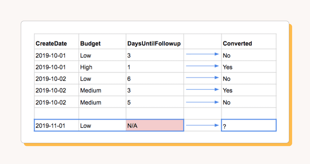
Here’s a simple illustration of the problem: let's say our leads dataset has the fields CreateDate, BudgetAmount, and DaysUntilFollowup, where DaysUntilFollowupis the number of days that elapsed between CreateDate and a sales person following up on each lead. And we know which of those leads eventually converted to sales.
We build a model using those three variables to guess whether new leads will convert, and it has 90% accuracy on historical data—excellent! The problem? When we try to apply the model to new leads, we realize that none of them actually has a value for DaysUntilFollowup; no salesperson has reached out yet because all the leads are brand new. Turns out our model is useless on new data, and the 90% accuracy was an illusion.
It's very common for data values to be updated as teams gain more information, such as incrementing a lead's "DaysUntilFollowup" every day until a salesperson follows up. But it's critical that this "future" information isn't used to predict outcomes for new data.
The best way to prevent target leakage is to snapshot your data. Usually this means that a static snapshot of your explanatory data is taken daily and stored where it can't be edited. This allows you to do whatever you want with your current data, such as creating an updated field like DaysUntilFollowup, but you can always "rewind" to see the exact information you knew on any day in the past.
In practice, many organizations don't snapshot their data. That doesn't make statistical analysis impossible; you just have to be extra careful that the explanatory variables only contain information that you would have known when each lead was initially generated.
3. Leads should be uniquely matchable to conversions.
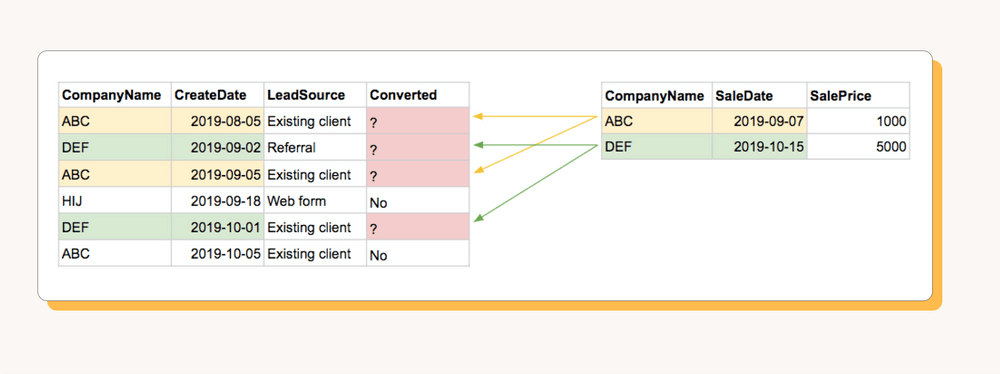
It may seem obvious that leads need to be matched to their final status (conversion or no conversion). In practice, though, there may not be a unique identifier that allows you to automatically match leads to conversions with no duplication. For example, let's say we have two tables: one for leads with the fields CompanyName, CreateDate, and LeadSource; another for conversions with the fields CompanyName, SaleDate, and SalePrice:
What happens when we try to determine whether each lead converted to a sale? If the same CompanyName has multiple leads or conversions, we'll have to infer from CreateDate and SaleDate which lead belongs to each conversion. What if we had to do this for thousands of leads? What if someone misspelled a CompanyName and it couldn't be matched to its conversion?
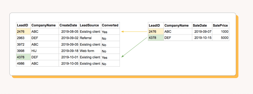
The best solution to this matching problem is to automatically generate a unique identifier for each new lead, which can be used across both tables to easily match leads to conversions. For example, if we had a field called LeadID, our matching problem would become much simpler:
4. There should be a way to identify currently-active leads.
Joining converted sales to our leads data tells us which leads successfully converted, but it doesn't necessarily tell us which leads definitely failed to convert.It's possible some of the leads in our dataset are still active and could become successful conversions in the future. If we include these active leads in our analysis and treat them as "failures", our model may draw incorrect conclusions about the relationships between our explanatory and outcome variables.
The best solution is to have some variable, for example CurrentLeadStatus, that we can use to drop active leads from the dataset. Note: to avoid target leakage, it's important that this status not be included as an explanatory variable in the model itself; it should only be used to filter the leads dataset.
If no such status variable exists, an alternative is to create some rule-of-thumb for how old our data has to be for us to consider it "final" for analysis. For example, say we have data on leads and conversions going back five years. We can calculate from the data that the vast majority (99%) of conversions happen within 60 days of lead generation. We could then reasonably exclude any leads generated in the last 60 days, since some of them may convert in the future, and only run our model on the older data. Note: This kind of data is known as censored data because the time until conversion occurs is unknown for some leads. Typically, survival analysis is used to model these kinds of censored time-to-event values. One way to approximate the cutoff in this case is to find the number of days X where X is the 99th percentile of days-until-sale among all leads generated more than X days ago.
5. Data on historical lead prioritization should exist.
Our last requirement for good lead-scoring data is the most subtle.
We want to build a model to predict which leads are most likely to convert to sales, and we have historical data that can be used to find these patterns. But what if our current way of prioritizing leads affects how likely certain leads are to convert? We might "contaminate" our model by having actively influenced past outcomes.
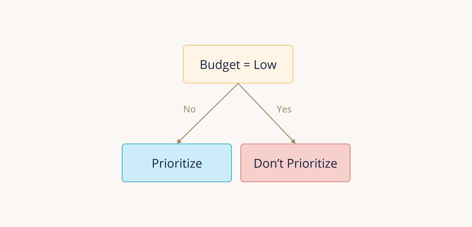
For example, let's say our current system for triaging leads tells us to put less sales effort into leads with small budgets:
The obvious outcome of devoting less effort to these leads is that they'll be less likely to convert. So when we build a model that includes budget as a variable, the algorithm will notice that leads with lower budgets are less likely to convert, and it will tell us to keep deprioritizing low-budget leads. The algorithm doesn't know that we effectively chose to make those leads convert at lower rates. But what if we were wrong? What if there are some scenarios where low-budget leads should be pursued, and we just didn't realize it?
This is known as selection bias. We've been selecting leads to be more likely to convert specifically because of their attributes (in this case, budget), rather than allowing the leads to convert or not without our influence. This makes it hard to tease out which attributes really affect conversion in a vacuum.
The gold standard to prevent selection bias is having some amount of randomized data. In other words, it's best to always set aside a small fraction of leads where sales effort is applied randomly or equally regardless of the kind of lead. Then we can study that data to avoid introducing our own biases into the model. However, most teams don't have the infrastructure or lead volume to continuously randomize a fraction of their leads.
Fortunately, data scientists have a few tools for dealing with non-random data:
Exclude leads with predetermined outcomes from the model. For example, if our current system auto-rejects all leads from outside the country, technically all those leads "fail to convert". An ML model will pick up on that and declare with extreme confidence that all leads from other countries are unlikely to convert. But those leads never had a chance of converting in the first place, so we should drop them from the model entirely.
Add a control variable to account for any influence our triaging system had on conversion probability. Using our example from above, where low-budget leads receive less sales effort, we can include some variable like AutoPrioritizationLevel to try to control for uneven sales effort applied to different kinds of leads.
⚠️ Note: to avoid target leakage, it's important that this control variable is one that would have been assigned as soon as the lead was generated.
What’s next?
So this is the end of part 1, hopefully this introduction to using machine learning to score leads has given you a primer on high level topics such as; what is a scoring model and when you need it or what type of data you need to build your model.
We're just getting started writing on this topic so I would love to hear your feedback on the article. If you have any questions, or are looking to use your data to do any type of scoring, from Product Lead Scoring to Account Health Scoring, get in touch with us. We've built scoring models for companies like Atrium, Vidyard and Notion!