Quick guide: SQL aggregate functions | Census

It’s universally known SQL is the language of data. Within this universal language, aggregate functions are an essential building block to help you summarize data, compute descriptive statistics quickly, and use more advanced functions, like window functions, to better process and understand data insights.

By the end of this article, you’ll have a solid grasp on five SQL aggregate functions you can use to improve your business operations, including:

• Function #1: COUNT()
• Function #2: COUNTIF()
• Function #3: SUM()
• Function #4: AVG()
• Function #5: MIN()/MAX()

I'll also cover the basics of what aggregate functions are, as well as how you do more with your data post-aggregation.

What are aggregate functions in SQL?

Aggregate functions are functions performed over one or more values. Generally, these functions return a single value, however, when they’re used alongside a GROUP BY clause, they can return one or more values.  You’ll have a better understanding of this after going through several real-world examples in this article.

There are five main types of aggregate functions that are essential for SQL coding:

1. COUNT()
2. COUNTIF()
3. SUM()
4. AVG()
5. MIN() / MAX()

For this article, we’re returning to our well-loved Sandy Shores example. 🏖️ Sandy Shores is a beach chair rental company that’s turning to data to get more insight into how their customers use their services, and where they can optimize their business model.

With that said, let’s dive into it!

1. COUNT()

COUNT returns the number of rows in a column, not including NULL values. If you wanted to only count the distinct number of values in a column, you could use COUNT(DISTINCT). For example, if you wanted to count the number of unique customers or the number of unique products, you would use COUNT(DISTINCT).

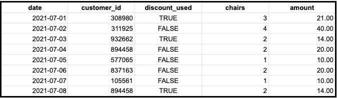
Let’s see how Sandy Shores might use these functions. Suppose Sandy Shores has the following table called transactions, which tracks transactions for chair rentals.

• date represents the date of the transaction
• customer_id represents a unique id for each distinct customer
• discount_used is TRUE if the customer used a discount and FALSE if not
• chairs represent the number of chairs that were rented
• amount represents the total amount of the transaction

The Sandy Shores team wants to get the total number of transactions from July 1 to July 8. They could run the following query:

SELECT COUNT(customer_id) FROM transactions

This would return the number of rows, which is equal to eight.

Simple right? What if team Sandy wanted to get the total number of unique customers?

SELECT COUNT(DISTINCT customer_id) FROM transactions

This would return seven because the customer with the id 894458 made two transactions, one on July 4 and one on July 8.

Pretty nice, right? Well, we can extend COUNT even further with the following function: COUNTIF()

2. COUNTIF()

COUNTIF is an extension of COUNT where it returns the number of rows that satisfy the condition.

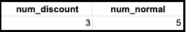
Let’s go back to our table, transactions. Suppose the folks at Sandy Shores wanted to count the number of transactions where a discount was used and the number of transactions where a discount wasn’t used. This would be a perfect time to use the COUNTIF function:

SELECT COUNTIF(discount_used = TRUE) as num_discount
, COUNTIF(discoun_used = FALSE) as num_normal
FROM transactions

This would return the following output:

Now the Sandy Shores team can easily see that nearly half of their customers are using their recent discount code, which can help inform how this discount type performs over others, or how discounts improve the overall number of customers during a given period.

3. SUM()

SUM returns the sum of non-null values — in other words, it adds up all of the values in a column. Don’t confuse this with COUNT. COUNT returns the number of rows in a column, while SUM adds up all of the values in a column.

There are several special cases when using SUM that you should know about:

• SUM() returns NULL if the column only has NULLs
• SUM() returns NULL if the column has no rows
• SUM() returns Inf/-Inf if the column contains Inf/-Inf
• SUM() returns NaN if the column contains a NaN
• SUM() returns NaN if the column has a combination of Inf and -Inf

SUM() is incredibly valuable when you want to know the total of ANYTHING. Let’s see how Sandy Shores can use SUM() to better understand their business.

Suppose team Sandy wanted to get the total amount that they made from July 1 to July 8. They  could simply run the following query:

SELECT SUM(amount)
FROM transactions

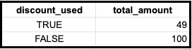
This would return a total of $149. What if they wanted to sum the total amount when a discount was applied vs. when it wasn’t so they could better understand the net cost/revenue of their discount campaign? Their code might look like this:

SELECT discount_used, SUM(amount) as total_amount
FROM transactions
GROUP BY discount_used

This would return the following:

The SUM function is a valuable tool in our toolbox to help us understand how much revenue or product we're selling at a given time, as well as a great way to narrow in on the performance of individual campaigns or sales.

4. AVG()

AVG simply returns the average of a column with non-null values. Mathematically speaking, AVG sums the values of a given column and then divides it by the corresponding number of rows.

AVG calculates a central tendency called the mean. This is extremely useful when you want to know how a particular metric is performing on average over time. For example, in a business setting you might want to know the following:

• You want to see if the average amount spent per transaction is growing over time
• You want to see if the average response time for your call center is decreasing
• You want to see if the average error rate for production is decreasing

Let’s see how Sandy Shores might use AVG to gain some insight into how their business performs over time.

For this example, the Sandy Shores team wants to figure out how many chair rentals the average customer has in early July. We’re working off the table below, which shows the rental date, customer ID, if they used a discount, how many chairs they rented, and the total rental cost for the day.

Based on the information we have in the table above, our code would look something like this:

SELECT AVG(chairs) as avg_chairs
, AVG(amount) as avg_amount
FROM transactions

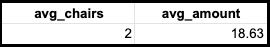
This query would return the following table with the average chairs rented per customer, and the average cost per customer per rental.

Awesome! Now the Sandy Shores team can better forecast future chair supply as they grow, and forecast earnings from their rentals, even when they’re offering discounts. Let’s take this one step further and check out our last function: MIN()/MAXI().

5. MIN() / MAX()

MIN and MAX simply return the minimum value and maximum value respectively for a column.

We previously went over AVG and how it provides the central tendency of a given column. MIN and MAX are very useful functions that complement AVG because they provide the range for a given column, allowing you to understand the variance as well as the mean.

Now, let’s get the MIN and MAX for chairs and amount, so the Sandy Shores team has a range of values for each, in addition to the average that their team already calculated:

SELECT MIN(chairs) as min_chairs
, MAX(chairs) as max_chairs
, MIN(amount) as min_amount
, MAX(amount) as max_amount
FROM transactions

This would result in the following:

Now the Sandy Shores team knows that they can expect an average of two chair rentals per customer with a minimum of one chair and a maximum of four chairs. Similarly, they can expect an average amount of $18.63 per rental order with a minimum of $10 and a maximum of $40. This data will be a great help when it comes to sales and inventory forecasting for future beach seasons.

What’s next: Doing more with your data

Now that you have a good understanding of aggregate functions, you’re ready to extend your knowledge even further. After all, you don't just want all this awesome, well-aggregated data to go die in a dashboard your business teams use once.

If you're ready to take the next step to do more with your data, learn more about reverse ETL, which breaks down how you can make the results of your data work available in every business tool your team uses (without engineering favors).

Or, if you're just on a mission to improve your SQL skills, check out some of the other great resources from the Census team here.