Terence is a data enthusiast and professional working with top Canadian tech companies. He received his MBA from Quantic School of Business and Technology and is currently pursuing a master's in computational analytics at Georgia Tech. Markham, Ontario, Canada
Key learnings from this article:
Types of fraud prediction models (and the differences between them)
Key features to use in your fraud prediction models
How to evaluate a fraud prediction model
As the world becomes more digitized and people are better equipped with new technologies and tools, the level of fraudulent activity continues to reach record-highs. According to a report from PwC, fraud losses totaled US$42 billion in 2020, affecting 47% of all companies in the past 24 months.
Paradoxically speaking, the same technological advancements, like big data, the cloud, and modern prediction algorithms, allows companies to tackle fraud better than ever before. In this article, we’re focused on the last point, fraud prediction algorithms - specifically, we’ll look at types of fraud models, features to use in a fraud model, and how to evaluate a fraud model.
Types of Fraud Prediction Models
“Fraud” is a wide-reaching, comprehensive term. So it should come as no surprise that you can build several types of fraud models, each serving its own purposes. Below, we’ll take a look at four of the most common models and map how they relate to each other.
Profile-specific models vs transaction-specific models
The idea of “innocent until proven guilty” isn’t just a concept for courtroom justice. It’s a philosophy that should ring true for your users to, and in order to ensure innocent folks aren’t put in digital jail because of the fraudulent actions of others you need to distinguish between the following two model types:
Profile-specific models, which focus on identifying fraudulent activity on a user level, meaning that these models determine whether a user is fraudulent or not.
Transaction-specific models, which take a more granular approach and identify fraudulent transactions, rather than fraudulent users.
At a glance, it sounds like these models serve the same purpose, but it’s not always the case that a fraudulent transaction comes from a fraudulent user. A user shouldn’t be deemed as fraudulent if his/her credit card was stolen and a fraudulent transaction was made on that credit card. Similarly, it’s not always the case that a fraudulent user makes a fraudulent transaction 100% of the time - whether that user should be allowed to make any transactions at all is a topic for another time.
Rules-based models vs machine learning models
If you’ve ever traveled across the country from your home and had your local bank freeze your credit card when you try to buy a cup of coffee at your destination, you know how annoying it can be when a bank uses rules-based models vs machine learning models.
Rules-based models are models with hard-coded rules, think of “if-else” statements (or case-when statements if you’re a SQL rockstar). With rules-based models, you’re responsible for coming up with the rules by yourself. Rules-based models are useful if you know the exact signals that indicate fraudulent activity. However, these models can be difficult if you either A) can't predict all fraudulent activity signals or B) can't guarantee those signals only correlate to fraudulent activity.
For example, credit card companies usually have a rules-based approach that checks the location of where you use your credit card. If the distance between where you spend your credit card and your home address location passes a certain threshold--if you’re too far away from home--the transaction may automatically be denied.
Machine learning fraud-detection models, on the other hand,have become increasingly popular with the emergence of data science over the past decade. Machine learning models shine when you don’t know the exact signals that indicate fraudulent activity. Instead, you provide a machine learning model with a handful of features (variables) and let the model identify the signals itself.
For example, banks feed dozens of engineered features into machine learning models to identify what transactions are likely to be fraudulent and are moved to a second stage for further investigation. This allows their ML model to learn which behaviors over others tend to signal fraudulent behavior over time.
Now that we’ve broken down the four popular fraud prediction models you should know, let’s take a look at the features they should have.
Key features to use in your model
When choosing the features for your fraud prediction model, you want to include as many signals indicating fraudulent activity as possible.
To help spark some ideas, here’s a non-exhaustive list of key features commonly used in machine learning models:
Time of registration or transaction: The time when a user registers or makes a transaction is a good signal because it gives you an idea of the normal operating hours of your users, which can help you identify fraudulent users who take suspicious action outside that window. This means that they may make a number of transactions at a time when people don’t normally make transactions.
Location of transaction: As I alluded to before, the location in which a transaction was made can sometimes indicate whether the transaction is fraudulent or not. If a transaction is made 2000 miles away from the home address within minutes of a closer-to-home transaction, that's abnormal behavior and can possibly be fraudulent.
Cost to average spend ratio: This looks at the amount of a given transaction compared to the average spend of the given user. The larger the ratio, the more irregular the transaction is (and more likely it's fraudulent).
Email information: You can actually check when an email account was created to flag it for potentially suspicious behavior (for example, if someone gets a potentially fraudulent email and the sender created the account earlier that day, it may suggest fraudulent behavior).
The more signals you can provide--and the stronger the signals are--the better your model can predict and identify fraudulent activity.
How to evaluate a fraud model
You have to evaluate a fraud model differently than normal machine learning models because the fraudulent activity is (hopefully) a very small slice of your overall sample data used to train models.
Why you shouldn’t use accuracy
Fraud detection is classified as an imbalanced classification problem. Specifically, there’s a significant imbalance between the number of fraudulent profiles/transactions and the number of non-fraudulent profiles/transactions. Because of this, you’re not going to get very far using accuracy as an evaluation metric.
To give an example of why, consider a dataset with one fraudulent transaction and 99 non-fraudulent transactions (in the real world, the ratio is even smaller). If a machine learning model were to classify every single transaction as non-fraudulent, it would be 99% accurate! Unfortunately, we’re not worried about non-fraudulent transactions and this accuracy-based model fails to tackle the problem at hand.
Metrics to use instead of accuracy
Instead, here are two metrics you should consider when evaluating a fraud-prediction model:
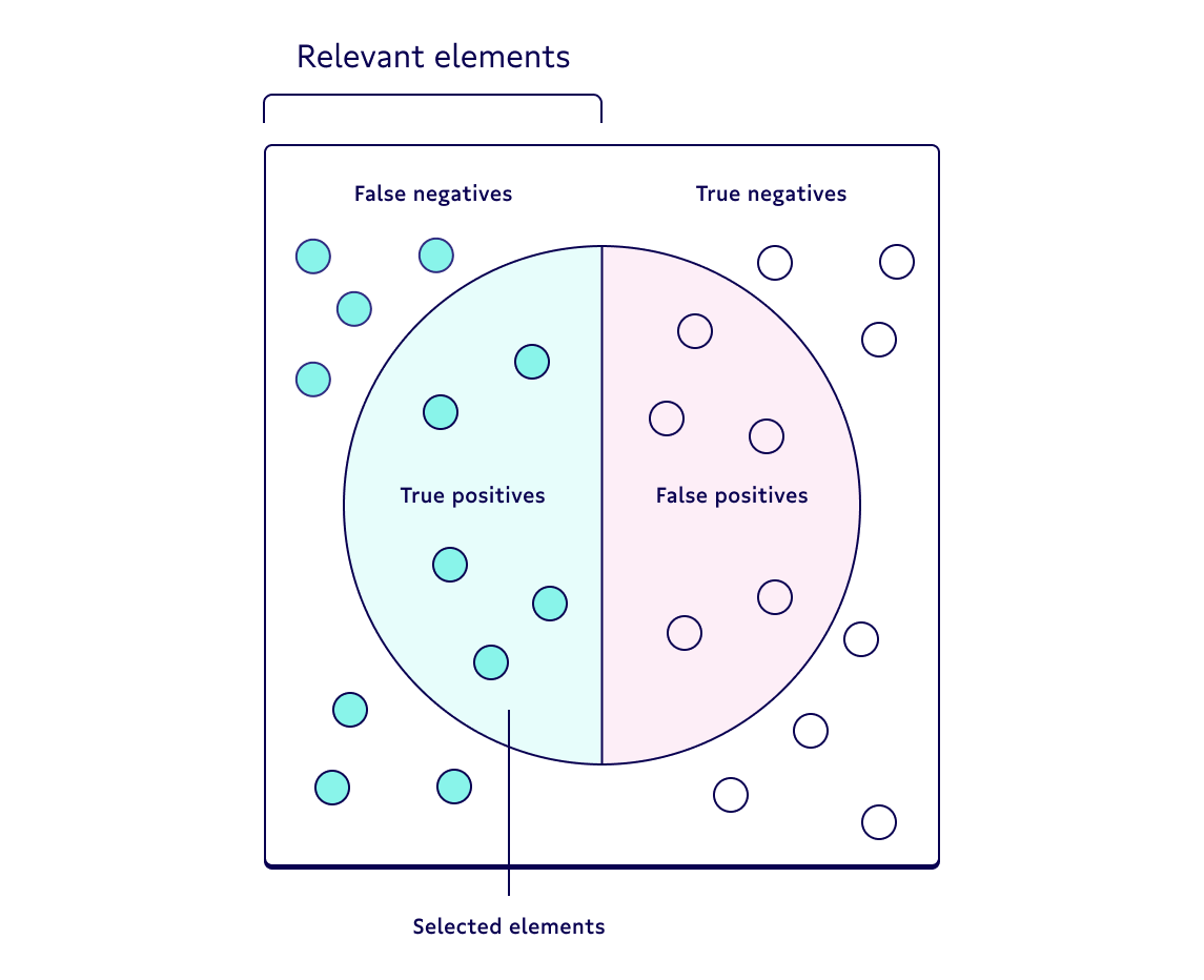
1. Precision, also known as a positive predictive value, is the proportion of relevant instances among the retrieved instances. In other words, it answers the question “What proportion of positive identifications was actually correct?”
You should use precision when the cost of classifying a non-fraudulent transaction as fraudulent is too high and you’re okay with only catching a portion of fraudulent transactions.
2. Recall--also known as the sensitivity, hit rate, or the true positive rate (TPR)--is the proportion of the total number of relevant instances that were actually retrieved. It answers the question “What proportion of actual positives was identified correctly?”
I recommend that you use recall when it’s absolutely critical you identify every single fraudulent transaction and you feel okay with incorrectly classifying some non-fraudulent transactions as fraudulent.
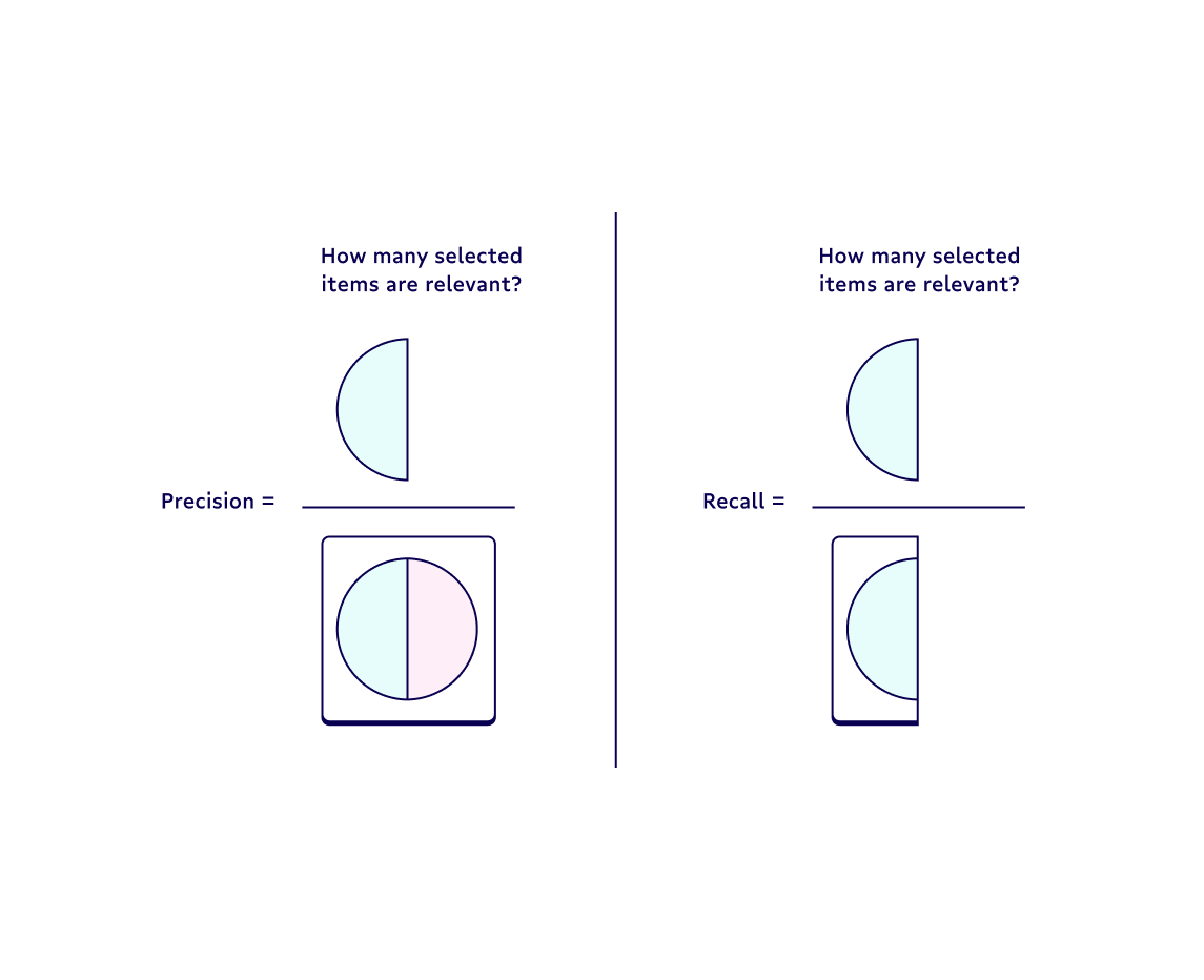
Each has its own pros and cons. You should weigh the strengths and weaknesses of each based on the business problem at hand. If you're a more visual person, check out the image below, which breaks down the difference between precision and recall metrics.
Take your knowledge further
Thanks for reading! You should now know about the types of fraud models, some key features that you can use in your model, and how to evaluate your fraud model.
Looking for even more ways to improve your data skills overall? Check out our other tutorials here. Or, if you have questions (or want help building and leveraging your fraud prediction models), drop us a line.