TABLE OF CONTENTS
How to Connect Snowflake with Python (Jupyter) Tutorial | Census

Parker is a data community advocate at Census with a background in data analytics. He's interested in finding the best and most efficient ways to make use of data, and help other data folks in the community grow their careers. Salt Lake City, Utah, United States

In this article, you’ll find a step-by-step tutorial for connecting Python with Snowflake. Specifically, you'll learn how to:
- How to connect Python (Jupyter Notebook) with your Snowflake data warehouse
- How to retrieve the results of a SQL query into a Pandas data frame
As always, if you're looking for more resources to further your data skills (or just make your current data day-to-day easier) check out our other how-to articles here.
If your title contains “data” or “engineer”, you likely have strict programming language preferences. Good news: Snowflake hears you! You can now connect Python (and several other languages) with Snowflake to develop applications. If you're a Python lover, here are some advantages of connecting Python with Snowflake:
- Optimize development time
- Improved machine learning and linear regression capabilities
- Accelerate operational analytics capabilities
In this tutorial, I'll run you through how to connect Python with Snowflake. Let's get into it.
Software requirements
First, you need to make sure you have all of the following programs, credentials, and expertise:
- A table in your Snowflake database with some data in it
- User name, password, and host details of the Snowflake database
- Jupyter Notebook
- Familiarity with Python and programming constructs
Next, we'll go to Jupyter Notebook to install Snowflake's Python connector.
Install Snowflake Connector for Python
The Snowflake Connector for Python gives users a way to develop Python applications connected to Snowflake, as well as perform all the standard operations they know and love. You can install the connector in Linux, macOS, and Windows environments by following this GitHub link, or reading Snowflake’s Python Connector Installation documentation.
To connect Snowflake with Python, you'll need the snowflake-connector-python connector (say that five times fast). You can install the package using a Python PIP installer and, since we're using Jupyter, you'll run all commands on the Jupyter web interface.
Before you go through all that though, check to see if you already have the connector installed with the following command:
pip show snowflake-connector-pythonHowever, if the package doesn’t already exist, install it using this command:
pip install snowflake-connector-pythonIf you followed those steps correctly, you'll now have the required package available in your local Python ecosystem. Next, we'll tackle connecting our Snowflake database to Jupyter Notebook by creating a configuration file, creating a Snowflake connection, installing the Pandas library, and, running our read_sql function.
Create a configuration file
To start off, create a configuration file as a nested dictionary using the following authentication credentials:
- Username: The username for your Snowflake account. You can find this by querying current_user() in a Snowflake worksheet.
- Password: The password used to log in to Snowflake.
- Host: The hostname of your Snowflake warehouse. Example: abc1234567.us-east-2
Here's an example of the configuration file python code:
conns = {'SnowflakeDB':{ 'UserName': 'python','Password':'Pythonuser1', 'Host':'ne79526.ap-south.1.aws'}}I created a nested dictionary with the topmost level key as the connection name SnowflakeDB. Then, I wrapped the connection details as a key-value pair. In the future, if there are more connections to add, I could use the same configuration file.
Now, we'll use the credentials from the configuration file we just created to successfully connect to Snowflake.
Create a Snowflake connection
First, we'll import snowflake.connector with install snowflake-connector-python (Jupyter Notebook will recognize this import from your previous installation). Next, create a Snowflake connector connection that reads values from the configuration file we just created using snowflake.connector.connect. The code will look like this:
#import the module
import snowflake.connector

#create the connection
connection = snowflake.connector.connect(
    user=conns['SnowflakeDB']['UserName']
    , password=conns['SnowflakeDB']['Password']
    , account=conns['SnowflakeDB']['Host'])
You've officially installed the Snowflake connector for Python! Now you can use the open-source Python library of your choice for these next steps. For this tutorial, I’ll use Pandas.
Install the Pandas library
You may already have Pandas installed. You can check by running print(pd._version_) on Jupyter Notebook. If it’s not already installed, run the following:
import pandas as pdOnce you have the Pandas library installed, you can begin querying your Snowflake database using Python and go to our final step.
Run read_sql function
read_sql is a built-in function in the Pandas package that returns a data frame corresponding to the result set in the query string. In this example query, we'll do the following:
- Call our Pandas package pd
- Running the read_sql package
- Writing a SQL query
- Specifying our Snowflake connection
The query and output will look something like this:
pd.read.sql("SELECT * FROM PYTHON.PUBLIC.DEMO WHERE FIRST_NAME IN ('Michael', 'José')", connection)
Congratulations! You've officially connected Snowflake with Python and retrieved the results of a SQL query into a Pandas data frame. You can now use your favorite Python operations and libraries on whatever data you have available in your Snowflake data warehouse. This will help you optimize development time, improve machine learning and linear regression capabilities, and accelerate operational analytics capabilities (more on that below).
How to accelerate operational analytics capabilities
Operational analytics is a type of analytics that drives growth within an organization by democratizing access to accurate, relatively real-time data. It requires moving data from point A (ideally, the data warehouse) to point B (day-to-day SaaS tools). This means your data isn't just trapped in a dashboard somewhere, getting more stale by the day. Instead, you're able to use Snowflake to load data into the tools your customer-facing teams (sales, marketing, and customer success) rely on every day.
Here are some of the high-impact use cases operational analytics unlocks for your company when you query Snowflake data using Python:
- Sending product data from the data warehouse to Zendesk to help customer success teams prioritize tickets.
- Sending marketing data from the data warehouse to Facebook to help marketers create highly-personalized ad campaigns.
- Sending product analytics data of free trial users to Salesforce to help sales reps identify high-probability deals.
Now, you can get started with operational analytics using the concepts we went over in this article, but there's a better (and easier) way to do more with your data. That was is reverse ETL tooling, which takes all the DIY work of sending your data from A to B off your plate. If you'd like to learn more, sign up for a demo or try the product for free!
And, of course, if you have any questions about connecting Python to Snowflake or getting started with Census, feel free to drop me a line anytime.


